参考:
[1]https://www.cnblogs.com/judejie/p/8999832.html
[2]https://blog.csdn.net/zouxy09/article/details/20319673
[3]https://blog.csdn.net/Snoopy_Yuan/article/details/63684219?utm_medium=distribute.pc_relevant.none-task-blog-BlogCommendFromMachineLearnPai2-2.nonecase&depth_1-utm_source=distribute.pc_relevant.none-task-blog-BlogCommendFromMachineLearnPai2-2.nonecase

完整代码:
(sklearn库实现)https://github.com/happybear1234/The-Watermelon-book-exercises/blob/master/Practical_3.3/code/Practical_3.3.py
(梯度下降实现)https://github.com/happybear1234/The-Watermelon-book-exercises/blob/master/Practical_3.3/code/Practical_3.3_self_def.py

习题3.3 编程实现对率回归,并给出西瓜数据集(如下)上的结果.

密度	含糖率	好瓜
0.697	0.46	是
0.774	0.376	是
0.634	0.264	是
0.608	0.318	是
0.556	0.215	是
0.403	0.237	是
0.481	0.149	是
0.437	0.211	是
0.666	0.091	否
0.243	0.267	否
0.245	0.057	否
0.343	0.099	否
0.639	0.161	否
0.657	0.198	否
0.36	0.37	否
0.593	0.042	否
0.719	0.103	否

因此将以上数据中好瓜表示为”1”,不好的瓜表示为”0”,转换成csv文件便于读取

公式说明

基础线性模型:
$$f(x)=\omega_{1}x_{1}+\omega_{2}x_{2}…+\omega_{d}x_{d}+b$$
可转化为向量:
$$f(x)={\omega}x^T+b$$
继而令$\beta=({\omega},b)$,$\hat{x}=(x,1)$,那么(注:此处均作为行向量,与西瓜书上相反,):
$$f(x)={\omega}x^T+b={\beta}\hat{x}^T$$
为了解决此处的二分类问题,将预测值映射成$y\in{0,1}$的值,即将线性回归转化为逻辑回归,常常采用以下的对数几率函数(sigmoid函数)代替:
$$y=\frac{1}{1+e^{-\beta\hat{x}^T}}$$
因此,只要求得$\omega$和$b$的值即可,以下通过极大似然法来估计$\omega$和$b$的值:
$$\psi(\beta)=\sum_{i=1}^{m}(y_{i}\beta\hat{x}^T_{i}-ln(1+e^{\beta\hat{x}^T_{i}}))$$
将上式最大化转化为最小化,便于后面梯度下降求解,如西瓜书P59公式3.27:
$$\psi(\beta)=\sum_{i=1}^{m}(-y_{i}\beta\hat{x}^T_{i}+ln(1+e^{\beta\hat{x}^T_{i}}))$$

该函数为连续可导凸函数(对应海塞矩阵正定),因此可用梯度下降求得最优解,梯度为:
$$\frac{\varphi\psi(\beta)}{\varphi\beta}=\sum_{i=1}^{m}(-y_{i}+\frac{1}{1+e^{-\beta\hat{x}^T}})\hat{x}_{i}$$
迭代过程(其中$\lambda$为步长)为:
$$\beta^{t+1}=\beta^{t}-\lambda\frac{\varphi\psi(\beta)}{\varphi\beta}$$

sklearn库实现

载入数据,预处理

import numpy as np
import matplotlib.pyplot as plt


dataset = np.loadtxt('/home/data/watermelon_3a.csv', delimiter=',')

X = dataset[:, 1 : 3]
y = dataset[:, 3]
print(np.shape(X))

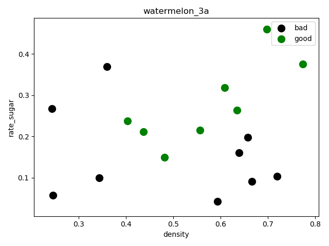
(17, 2)

绘制分散图,查看数据分散情况:

f1 = plt.figure(1)
plt.title('watermelon_3a')
plt.xlabel('density')
plt.ylabel('rate_sugar')
plt.scatter(X[y == 0, 0], X[y == 0, 1], marker = 'o', color = 'k', s = 100, label= 'bad')
plt.scatter(X[y == 1, 0], X[y ==1, 1], marker= 'o', color = 'g', s = 100, label = 'good')
plt.legend(loc = 'upper right')
plt.show()

sklearn逻辑回归库拟合

调用sklearn中的逻辑回归模型进行训练和预测

from sklearn import model_selection
from sklearn.linear_model import LogisticRegression
from sklearn import metrics
import matplotlib.pylab as pl

# 切分数据集:留出法 返回 划分好的训练集测试集样本和训练集测试集标签
X_train, X_test, y_train, y_test = model_selection.train_test_split(X, y, test_size=0.5, random_state=0)

# 训练模型
log_model = LogisticRegression()
log_model.fit(X_train, y_train)

# 模型测试
y_pred = log_model.predict(X_test)

打印混淆矩阵和相关度量,结果如下:

1
2
3

print(metrics.confusion_matrix(y_test, y_pred))
print(metrics.classification_report(y_test, y_pred))
precision, recall, thresholds = metrics.precision_recall_curve(y_test, y_pred)

[[3 2]
 [1 3]]

precision    recall  f1-score   support

     0.0       0.75      0.60      0.67         5
     1.0       0.60      0.75      0.67         4

    accuracy                           0.67         9
   macro avg       0.68      0.68      0.67         9
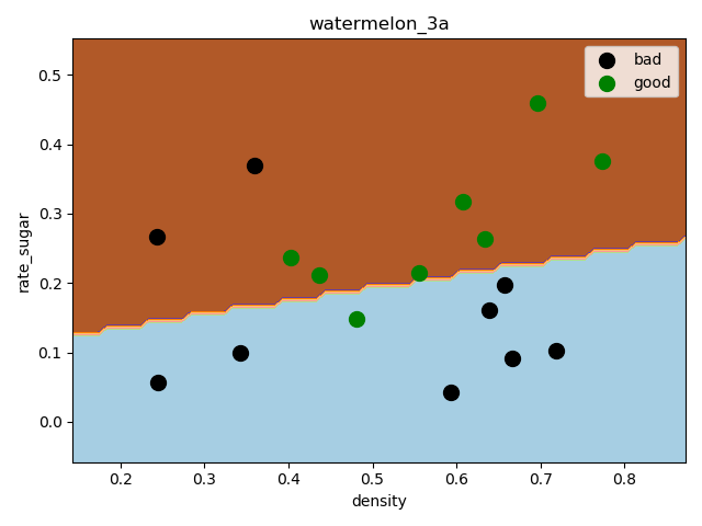
weighted avg       0.68      0.67      0.67         9

这里选择的留出法抽取样本,因为样本比较少,拟合效果一般,预测精度只有67%,可以采用自助法或者交叉验证法重新抽样,进一步选择最优模型

绘制决策边界

f2 = plt.figure(2)
h = 0.01
x0_min, x0_max = X[:, 0].min() - 0.1, X[:, 0].max() + 0.1
x1_min, x1_max = X[:, 1].min() - 0.1, X[:, 1].max() +0.1
x0, x1= np.meshgrid(np.arange(x0_min, x0_max, h), np.arange(x1_min, x1_max, h)) # 生成笛卡尔积坐标矩阵

z = log_model.predict(np.c_[x0.ravel(), x1.ravel()]) # c_ 按列合并, ravel 降成一维

z = z.reshape(x0.shape)
plt.contourf(x0, x1, z, cmap = pl.cm.Paired)# 等高线

plt.title('watermelon_3a')
plt.xlabel('density')
plt.ylabel('rate_sugar')
plt.scatter(X[y==0, 0], X[y==0, 1], marker='o', color='k', s=100, label='bad')
plt.scatter(X[y==1, 0], X[y==1, 1], marker='o', color='g', s=100, label='good')
plt.legend(loc='upper right')
plt.show()

可以看出训练出来的分类器还是可以分类出大多数示例

梯度下降法实现

实现以上公式

# 1)实现 P59 公式3.27极大似然法

def likelihood_sub(x, y, beta):
    """
    :param x: 一个示例变量(行向量)
    :param y:一个样品标签(行向量)
    :param beta:3.27中矢量参数(行向量)
    :return: 单个对数似然 3.27
    """
    return -y * np.dot(beta, x.T) + np.math.log(1 + np.math.exp(np.dot(beta, x.T)))

def likelihood(X, y, beta):
    """
    公式 3.27 :对数似然函数(交叉熵损失函数)
    :param X: 示例变量矩阵
    :param y:样本标签矩阵
    :param beta:3.27中的矢量参数
    :return: beta 的似然值
    """
    sum = 0
    m, n = np.shape(X)

    for i in range(m):
        sum += likelihood_sub(X[i], y[i], beta)
    return sum

# 2)实现似然公式一阶偏导
def sigmoid(x, beta):
    """
    基础模型 S 形函数
    P59 对数几率回归(逻辑回归)公式 3.23
    :param x: 预测变量
    :param beta: beta 变量
    :return:S 形函数
    """
    return 1 / (1 + np.math.exp(- np.dot(beta, x.T)))
def partial_derivative(X, y, beta):
    """
    P60 似然公式一阶偏导3.30
    :param X:示例变量矩阵
    :param y:样本标签矩阵
    :param beta:3.27 中矢量参数
    :return: beta 的偏导数,梯度
    """
    m, n = np.shape(X)
    pd = np.zeros(n)

    for i in range(m):
        tmp = -y[i] + sigmoid(X[i], beta)
        for j in range(n):
            pd[j] += X[i][j] * tmp
    return pd

这里采用批量梯度下降法:

def gradDscent(X, y, alpha, iterations, n):
    """
    :param X:变量矩阵
    :param y:样本标签数组
    :return:3.27中beta参数最优解
    """
    cost = np.zeros(iterations) # 构建 max_times 个 0 的数组
    beta = np.mat(np.zeros(n)) # 初始化 beta

    for i in range(iterations):
        # 梯度下降
        output = partial_derivative(X, y, beta)
        beta = beta - alpha * output
        cost[i] = likelihood(X, y, beta)

    return beta, cost

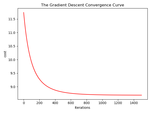
绘制收敛曲线

def showConvergCurve(Iterations, Cost):
    """
    :param Iterations: 迭代次数
    :param Cost: 损失值数组
    """
    f1 = plt.figure(1)
    t = np.arange(Iterations)
    p1 = plt.subplot(1,1,1)
    p1.plot(t, Cost, 'r')
    p1.set_xlabel('Iterations')
    p1.set_ylabel('cost')
    p1.set_title('The Gradient Descent Convergence Curve')

    plt.show()

这里步长取得0.1,迭代次数1500,在800次迭代后趋于稳定

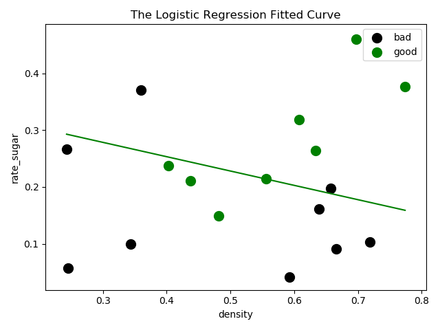
绘制决策边界

def showLogRegression(X, y, Beta, N):
    f2 = plt.figure(2)

    plt.title('The Logistic Regression Fitted Curve')
    plt.xlabel('density')
    plt.ylabel('rate_sugar')
    # f = Beta * X.transpose()
    # plt.plot(X[:, 2], f.tolist()[0], 'r', label = 'Prediction')
    min_x = min(X[:, 0])
    max_x = max(X[:, 0])
    y_min_x = (- Beta.tolist()[0][2] - Beta.tolist()[0][0] * min_x) / Beta.tolist()[0][1] # 由线性模型 y =  w1 * x1 + w2 * x2 +b
    y_max_x = (- Beta.tolist()[0][2] - Beta.tolist()[0][0] * max_x) / Beta.tolist()[0][1]
    plt.plot([min_x, max_x], [y_min_x, y_max_x], '-g')
    plt.scatter(X[y == 0, 0], X[y == 0, 1], marker='o', color='k', s=100, label='bad')
    plt.scatter(X[y == 1, 0], X[y == 1, 1], marker='o', color='g', s=100, label='good')
    plt.legend(loc='upper right')
    plt.show()

看上去并没有sklearn库中逻辑回归分类器效果好,但是计算出来的精度却比分类器要高(这里为了方便没有划分数据集,可以重新用sklearn分好的数据再做对比)

测试

def testLogRegres(Beta, test_x, test_y):
    m, n = np.shape(test_x)
    matchCount = 0
    for i in range(m):
        predict = sigmoid(test_x[i], Beta) > 0.5
        if predict == bool(test_y[i]):
            matchCount += 1
    accuracy = float(matchCount) / m
    return accuracy

def loadData():
    dataset = np.loadtxt('/home/data/watermelon_3a.csv', delimiter=',')

    X = dataset[:, 1: 3]
    tmp = np.ones(X.shape[0])
    X = np.insert(X, 2, values=tmp, axis=1) # 在最后一列插入全是 1 的列
    y = dataset[:, 3]
    return X, y

def main():
    alpha = 0.1  # 迭代步长
    iterations = 1500  # 迭代次数上限
    X, y = loadData()
    test_x = X
    test_y = y
    m, n = np.shape(X)
    beta, cost = gradDscent(X, y, alpha, iterations, n)
    print(beta)
    showConvergCurve(iterations, cost)
    showLogRegression(X, y, beta, n)
    accuracy = testLogRegres(beta, test_x, test_y)
    print('The classify accuracy is: %.3f%%' %(accuracy * 100))

The classify accuracy is: 70.588%