1
2
3
4
5
6
7
8
9
10
11
12
13
14
15
16
17
18
19
20
21
22
23
24
25
26
27
28
29
30
31
32
33
34
35
36
37
38
39
40
41
42
43
44
45
46
47
48
49
50
51
52
53
54
55
56
57
58
59
60
61
62
63
64
65
66
67
68
69
70
71
72
73
74
75
76
77
78
79
80
81
82
83
84
85
86
87
88
89
90
91
92
93
94
95
96
97
98
99
100
101
102
103
104
105
106
107
108
109
110
111
112
113
114
115
116
117
118
119
120
121
122
123
124
125
126
127
128
129
130
131
132
133
134
135
136
137
138
139
140
141
142
143
144
145
146
147
148
149
150
151
152
153
154
155
156
157
158
159
160
161
162
163
164
165
166
167
168
169
170
171
172
173
174
175
176
177
178
179
180
181
182
183
184
185
186
187
188
189
190
191
192
193
194
195
196
197
198
199
200
201
202
203
204
205
206
207
208
209
210
211
212
213
214
215
216
217
218
219
220
221
222
223
224
225
226
227
228
229
230
231
232
233
234
235
236
237
238
239
240
241
242
243
244
245
246
247
248
249
250
251
252
| import pandas as pd
import numpy as np
import matplotlib.pyplot as plt
import seaborn as sns
from operator import itemgetter
# %matplotlib inline 在终端中可以代替plt。show() 直接生成图
Train_data = pd.read_csv("./datalab/used_car_train_20200313.csv", sep=" ")
Test_data = pd.read_csv("./datalab/used_car_testA_20200313.csv", sep=" ")
# print(Train_data.shape)
# print(Train_data.head())
#print(Train_data.columns)
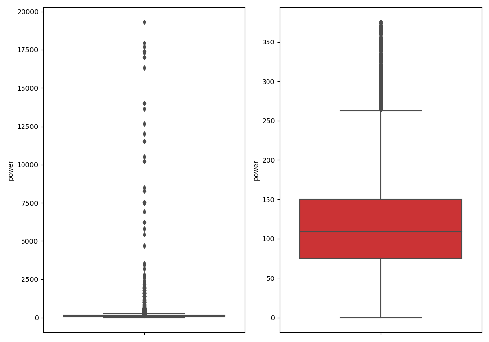
## 删除异常值
# 这里我包装了一个异常值处理的代码,可以随便调用
def outliers_proc(data, col_name, scale=3):
"""
用于清洗异常值,默认用box_plot(scale=3)进行清洗
:param data:接受 pandas 数据格式
:param col_name:pandas 列名
:param scale:尺度
"""
def box_plot_outliers(data_ser, box_scale):
"""
利用箱线图去除异常值
:param data_ser:接收 pandas.Series 数据格式
:param box_scale: 箱线图尺度 (规定大于上四分位数1.5倍四分位数差 的值,或者小于下四分位数1.5倍四分位数差的值,划为异常值)
"""
iqr = box_scale * (data_ser.quantile(0.75) - data_ser.quantile(0.25)) # 3倍四分位数差
val_low = data_ser.quantile(0.25) - iqr # 下限=Q1-3IQR
val_up = data_ser.quantile(0.75) + iqr # 上限=Q3+3IQR
rule_low = (data_ser < val_low)
rule_up = (data_ser > val_up) # 返回 pandas.Series 中对应值的bool
return (rule_low, rule_up), (val_low, val_up)
data_n = data.copy() # copy 数据
data_series = data_n[col_name] # 返回指定 col_name 数据
rule, value = box_plot_outliers(data_series, box_scale=scale)
index = np.arange(data_series.shape[0])[rule[0]|rule[1]] # 返回rule_low, rule_up中为True的下标的列表
#print("Delete number is:{}".format(len(index))) # 打印下标列表中个数
data_n = data_n.drop(index) # 删除(删除后下标没变)
data_n.reset_index(drop=True, inplace=True) # 重置索引(drop=True删除原来的索引;inplace=True当前修改状态应用到原来Series中)
#print("Now column number is:{}".format(data_n.shape[0])) # 查看删除后的数据个数
index_low = np.arange(data_series.shape[0])[rule[0]]
outliers = data_series.iloc[index_low] # ilco-按下标进行索引
#print("Description of data larger than the lower bound is:")
#print(pd.Series(outliers).describe())
index_up = np.arange(data_series.shape[0])[rule[1]]
outliers = data_series.iloc[index_up]
#print("Description of data larger than the upper bound is:")
#print(pd.Series(outliers).describe())
#fig, ax = plt.subplots(1, 2, figsize=(10, 7)) # 创建子图:1行2列
#sns.boxplot(y=data[col_name], data=data, palette="Set1", ax=ax[0]) # 箱线图
#sns.boxplot(y=data_n[col_name], data=data_n, palette="Set1", ax=ax[1])
#plt.show()
return data_n
## 我们可以删掉一些异常数据,以 power 为例
## 这里删不删可以自行判断
## 但是注意 Test 的数据不能删
Train_data = outliers_proc(Train_data, "power", scale=3)
## 特征构造
# 训练集和测试集放在一起,方便构造特征
Train_data["train"] = 1 # 添加新字段,并设置值为1
Test_data["train"] = 1
data = pd.concat([Train_data,Test_data],ignore_index=True) # 连接函数 ignore_index=True重置索引
# 使用时间:data["createDate"] - data["regDate"], 反应汽车使用时间,一般来说价格与使用时间成反比
# 不过要注意, 数据里有时间出错的格式, 所以我们需要 errors = "coerce"
data["used_time"] = (pd.to_datetime(data["creatDate"], format="%Y%m%d", errors="coerce") -
pd.to_datetime(data["regDate"],format="%Y%m%d",errors="coerce")).dt.days # to_datetime将参数转换为日期 dt.days每个元素的天数
# 看一下空数据, 有 15k 个样本的时间有问题的, 我们可以选择删除, 也可以选择放着
# 但是这里不建议删除, 因为删除缺失数据占总样本量过大, 7.5%
# 我们可以先放着, 因为如果我们 XGBoost 之类的决策树, 其本身就能处理缺失值, 所以可以不用管
#print(data["used_time"].isnull().sum())
# 从邮编中提取城市信息, 相当于加入了先验知识
#print(data["regionCode"])
# 增加city 字段, 并从 regionCode 值的倒数第三位切片(apply 对regionCode每个元素运行指定运算 lambda 匿名函数)
data["city"] = data["regionCode"].apply(lambda x : str(x)[:-3])

# 计算某品牌的销售统计量, 还可以计算其他特征的统计量
# 这里以 train 的数据计算统计量
Train_gb = Train_data.groupby("brand") # 分组
all_info = {}
for kind, kind_data in Train_gb:
    info = {}
    kind_data = kind_data[kind_data["price"] > 0]
    info["brand_amount"] = len(kind_data)
    info["brand_price_max"] = kind_data.price.max()
    info["brand_price_median"] = kind_data.price.median()
    info["brand_price_min"] = kind_data.price.min()
    info["brand_price_sum"] = kind_data.price.sum()
    info["brand_price_std"] = kind_data.price.std() # 样本方差
    info["brand_price_average"] = round(kind_data.price.sum() / (len(kind_data)+1), 2) # round(2)取近似值保留两位数
    all_info[kind] = info

brand_fe = pd.DataFrame(all_info).T.reset_index().rename(columns={"index":"brand"}) # T转置   reset_index还原索引  rename并修改列名
data = data.merge(brand_fe, how="left", on="brand") # 合并数据 data链接在brand_fe "brand"字段左边
# 数据分桶 以 power 为例
# 这时候缺失值也进桶了
# 为什么要分桶:
# 1. 离散后稀疏向量内积乘法运算速度更快, 计算结果也方便存储, 容易扩展
# 2. 离散后的特征对异常值更具鲁棒性, 如 age>30 为 1 否则为 0 , 对于年龄为 200 的也不会对模型造成很大的干扰
# 3. LR 属于广义线性模型, 表达能力有限, 经过离散化后, 每个变量有单独的权重, 这相当于引入了非线性, 能够提升模型的表达能力, 加大拟合
# 4. 离散后特征可以进行特征交叉, 提升表达能力, 由 M+N 个变量变成 M*N 个变量, 进一步引入非线性, 提升了表达能力
# 5. 特征离散后模型更稳定, 如用户年龄区间, 不会因为用户年龄长了一岁就变化
# 当然还有很多原因, LightGBM 在改进 XGBoost 时就增加了数据分桶, 增强了模型的泛化性
bin = [i*10 for i in range(31)]
data["power_bin"] = pd.cut(data["power"], bin, labels=False) # 分桶 cut切分数据(必须是一维的) bin定义区间 labels=False返回第几个bin(从0开始)
#print(data[["power_bin", "power"]].head())
# 删除不需要的数据
data = data.drop(["creatDate", "regDate", "regionCode"], axis=1) # drop函数默认删除行,列需要加axis = 1
#print(data.shape)
#print(data.columns)
# 目前的数据其实已经可以给树模型使用了, 所以我们导出一下
#data.to_csv("data_for_tree.csv", index=0) # index=0不保存行索引
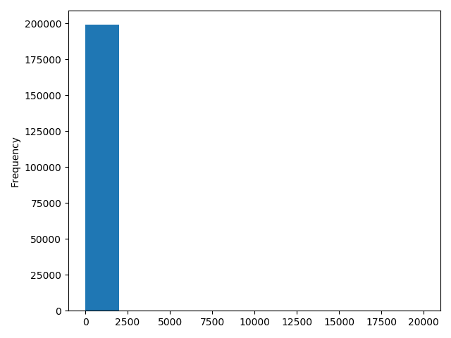
# 我们可以再构造一份特征给 LR NN 之类的模型用
# 之所以分开构造是因为, 不同模型对数据的要求不同
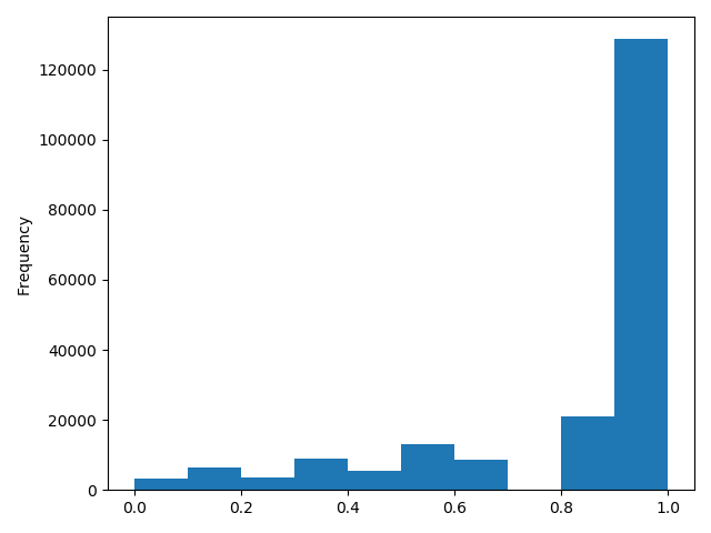
# 先看下数据分布:
#data["power"].plot.hist()
#plt.show()
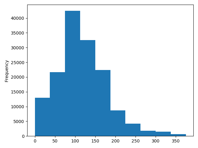
# 我们刚刚已经对 train 进行异常值处理了,但是现在还有这么奇怪的分布是因为 test 中的 power 异常值,
# 所以我们其实刚刚 train 中的 power 异常值不删为好,可以用长尾分布截断来代替
#Train_data["power"].plot.hist()
#plt.show()
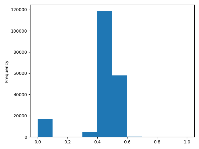
# 我们对其取 log, 再做归一化
from sklearn import preprocessing
# 将数据的每一个特征缩放到给定的范围,将数据的每一个属性值减去其最小值,然后除以其极差(最大值 - 最小值)
min_max_scaler = preprocessing.MinMaxScaler()
data["power"] = np.log(data["power"] + 1)
# 归一化:(0,1)标准化
data["power"] = ((data["power"] - np.min(data["power"])) / (np.max(data["power"]) - np.min(data["power"])))
#data["power"].plot.hist()
#plt.show()
# km 的比较正常, 应该已经做过分桶了
# data["kilometer"].plot.hist()
# plt.show()
# 所以可以直接作归一化
data["kilometer"] = ((data["kilometer"] - np.min(data["kilometer"])) /
(np.max(data["kilometer"]) - np.min(data["kilometer"])))
#data["kilometer"].plot.hist()
#plt.show()
# 除此之外 还有我们刚刚构造的统计量特征:
# 'brand_amount', 'brand_price_average', 'brand_price_max',
# 'brand_price_median', 'brand_price_min', 'brand_price_std',
# 'brand_price_sum'
# 这里不再一一举例分析了,直接做变换,
def max_min(x):
return (x - np.min(x)) / (np.max(x) - np.min(x))
data['brand_amount'] = ((data['brand_amount'] - np.min(data['brand_amount'])) /
(np.max(data['brand_amount']) - np.min(data['brand_amount'])))
data['brand_price_average'] = ((data['brand_price_average'] - np.min(data['brand_price_average'])) /
(np.max(data['brand_price_average']) - np.min(data['brand_price_average'])))
data['brand_price_max'] = ((data['brand_price_max'] - np.min(data['brand_price_max'])) /
(np.max(data['brand_price_max']) - np.min(data['brand_price_max'])))
data['brand_price_median'] = ((data['brand_price_median'] - np.min(data['brand_price_median'])) /
(np.max(data['brand_price_median']) - np.min(data['brand_price_median'])))
data['brand_price_min'] = ((data['brand_price_min'] - np.min(data['brand_price_min'])) /
(np.max(data['brand_price_min']) - np.min(data['brand_price_min'])))
data['brand_price_std'] = ((data['brand_price_std'] - np.min(data['brand_price_std'])) /
(np.max(data['brand_price_std']) - np.min(data['brand_price_std'])))
data['brand_price_sum'] = ((data['brand_price_sum'] - np.min(data['brand_price_sum'])) /
(np.max(data['brand_price_sum']) - np.min(data['brand_price_sum'])))
# 对类别特征进行 OneEncoder
data = pd.get_dummies(data, columns=['model', 'brand', 'bodyType', 'fuelType',
'gearbox', 'notRepairedDamage', 'power_bin']) # 装换虚伪变量
#print(data.shape)
#print(data.columns)
# 这份数据可以给 LR 用
#data.to_csv("data_for_lr.csv", index=0)
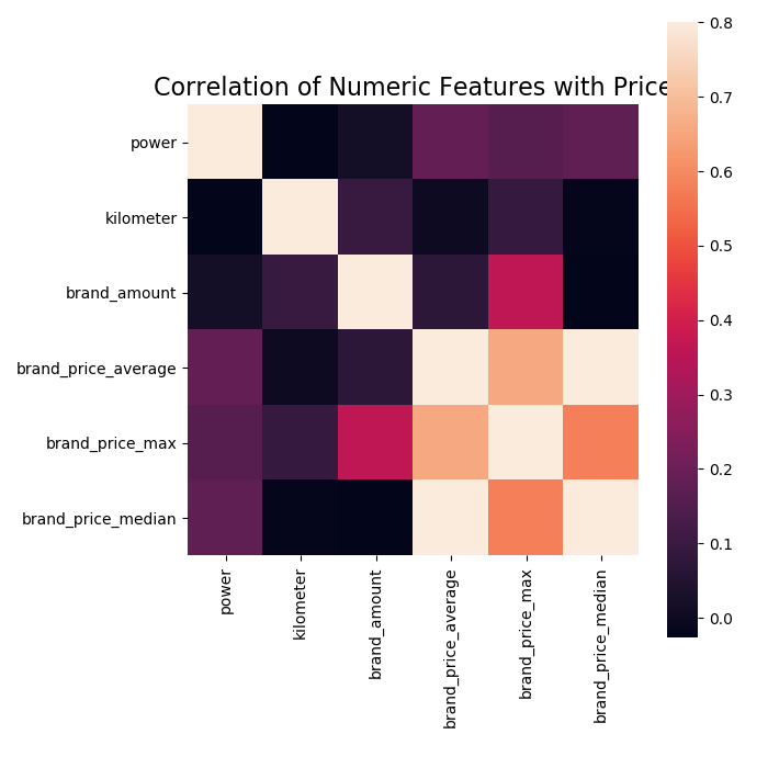
# 特征筛选
# 1)过滤式
# 相关性分析
# print(data['power'].corr(data['price'], method='spearman')) #spearman:非线性的,非正太分析的数据的相关系数
# print(data['kilometer'].corr(data['price'], method='spearman'))
# print(data['brand_amount'].corr(data['price'], method='spearman'))
# print(data['brand_price_average'].corr(data['price'], method='spearman'))
# print(data['brand_price_max'].corr(data['price'], method='spearman'))
# print(data['brand_price_median'].corr(data['price'], method='spearman'))
# 当然也可以直接看图
# data_numeric = data[['power', 'kilometer', 'brand_amount', 'brand_price_average',
# 'brand_price_max', 'brand_price_median']]
# correlation = data_numeric.corr() #返回data_numeric 相关性矩阵
#
# f, ax = plt.subplots(figsize=(7,7))
# plt.title("Correlation of Numeric Features with Price", y=1, size=16)
# square=True # 将坐标轴方向设置为“equal”,以使每个单元格为方形 , vmax:色彩映射的值
# sns.heatmap(correlation, square=True, vmax=0.8)
# plt.show()
# # 2)包裹式
from mlxtend.feature_selection import SequentialFeatureSelector as SFS #序列特征算法的实现——贪婪搜索算法
from sklearn.linear_model import  LinearRegression # 基于最小二乘法的线性回归
sfs = SFS(LinearRegression(), # 分类器或回归矩阵
          k_features=10, # 要选择的特征数量
          forward=True, #  如果为True,则向前选择,否则为反向选择
          floating=False, # 如果为True,则添加条件排除/包含。
          scoring="r2", # 对于sklearn回归变量使用“ r2”
          cv=0) # 如果cv为None、False或0,则不进行交叉验证
x = data.drop(["price"], axis=1)
x = x.fillna(0)
y = data["price"]

sfs.fit(x, y) # 执行特征选择并从训练数据中学习模型 x训练样本 y目标值
sfs.k_feature_names_


# 画出来,可以看到边际效益
from mlxtend.plotting import plot_sequential_feature_selection as plot_sfs
import matplotlib.pyplot as plt
fig1 = plot_sfs(sfs.get_metric_dict(), kind='std_dev')
plt.grid()
|