1
2
3
4
5
6
7
8
9
10
11
12
13
14
15
16
17
18
19
20
21
22
23
24
25
26
27
28
29
30
31
32
33
34
35
36
37
38
39
40
41
42
43
44
45
46
47
48
49
50
51
52
53
54
55
56
57
58
59
60
61
62
63
64
65
66
67
68
69
70
71
72
73
74
75
76
77
78
79
80
81
82
83
84
85
86
87
88
89
90
91
92
93
94
95
96
97
98
99
100
101
102
103
104
105
106
107
108
109
110
111
112
113
114
115
116
117
118
119
120
121
122
123
124
125
126
127
128
129
130
131
132
133
134
135
136
137
138
139
140
141
142
143
144
145
146
147
148
149
150
151
152
153
154
155
156
157
158
159
160
161
162
163
164
165
166
167
168
169
170
171
172
173
174
175
176
177
178
179
180
181
182
183
184
185
186
187
188
189
190
191
192
193
194
195
196
197
198
199
200
201
202
203
204
205
206
207
208
209
210
211
212
213
214
215
216
217
218
219
220
221
222
223
224
225
226
227
228
229
230
231
232
233
234
235
236
237
238
239
240
241
242
243
244
245
246
247
248
249
250
251
252
253
254
255
256
257
258
259
260
261
262
263
264
265
266
267
268
269
270
| # 导入warnings包,利用过滤器来实现忽略警告语句
import warnings
warnings.filterwarnings("ignore")
import pandas as pd
import numpy as np
import matplotlib.pyplot as plt
import seaborn as sns
import missingno as msno
## pd.set_option('display.max_columns', None)# 显示所有列
## pd.set_option('display.max_row', None)# 显示所有行
## 1)载入训练集和测试集
Train_data = pd.read_csv("./datalab/used_car_train_20200313.csv", sep = " ")
Test_data = pd.read_csv("./datalab/used_car_testA_20200313.csv", sep = " ")
## 2)简略观察数据(head()+shape)
#print(Train_data.head().append(Train_data.tail()))
#print(Train_data.shape)
#
# ## 3)通过describe()来熟悉相关统计量
# print(Train_data.describe())
#
# ## 4)通过info()来熟悉数据类型
# print(Train_data.info())
#
# ## 5)判断数据缺失和异常
# print(Train_data.isnull().sum())
#
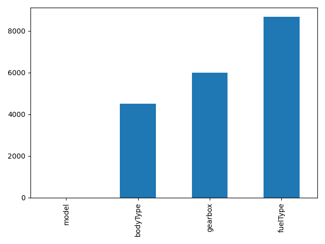
#nan可视化
# missing = Train_data.isnull().sum()
# missing = missing[missing > 0]
# missing.sort_values(inplace=True) # 排序
# missing.plot.bar() # 绘柱状图
# plt.tight_layout() # 自动调整子图参数
# plt.show()
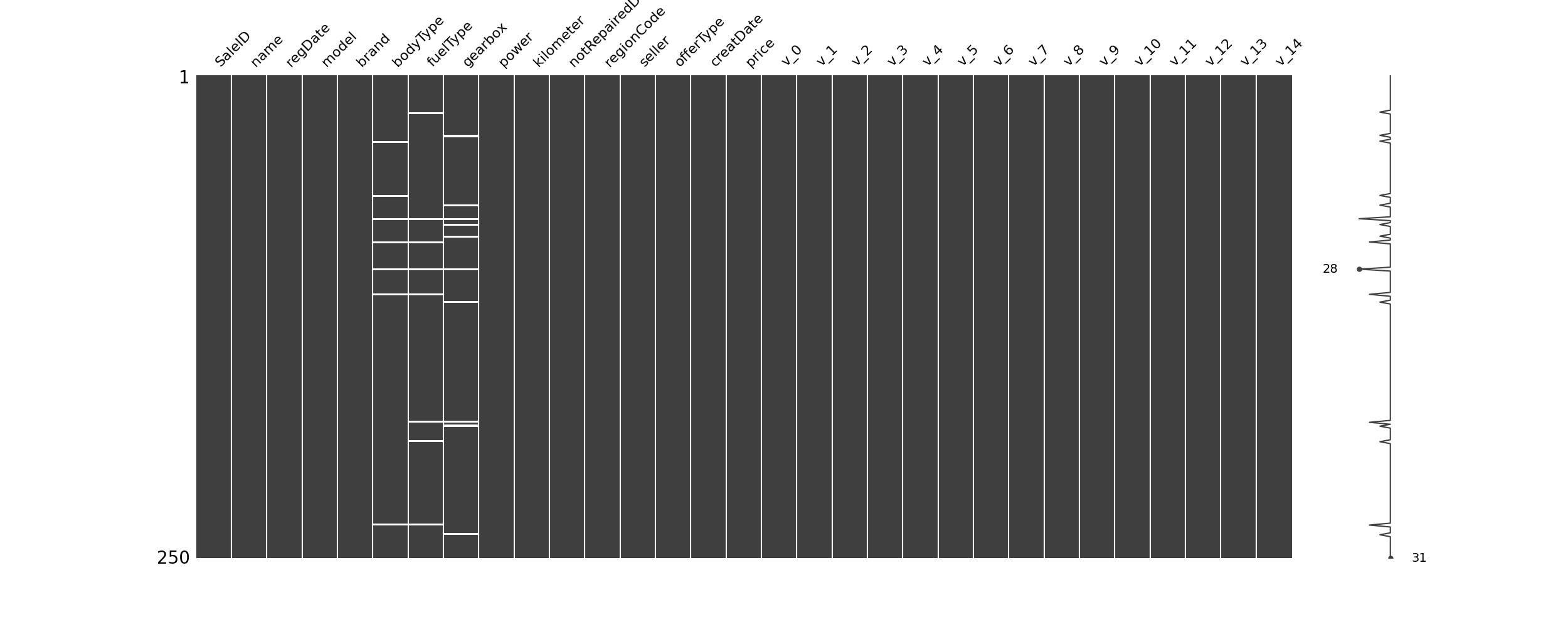
# # # 可视化看下缺省值
# msno.matrix(Train_data.sample(250))
# # plt.show()
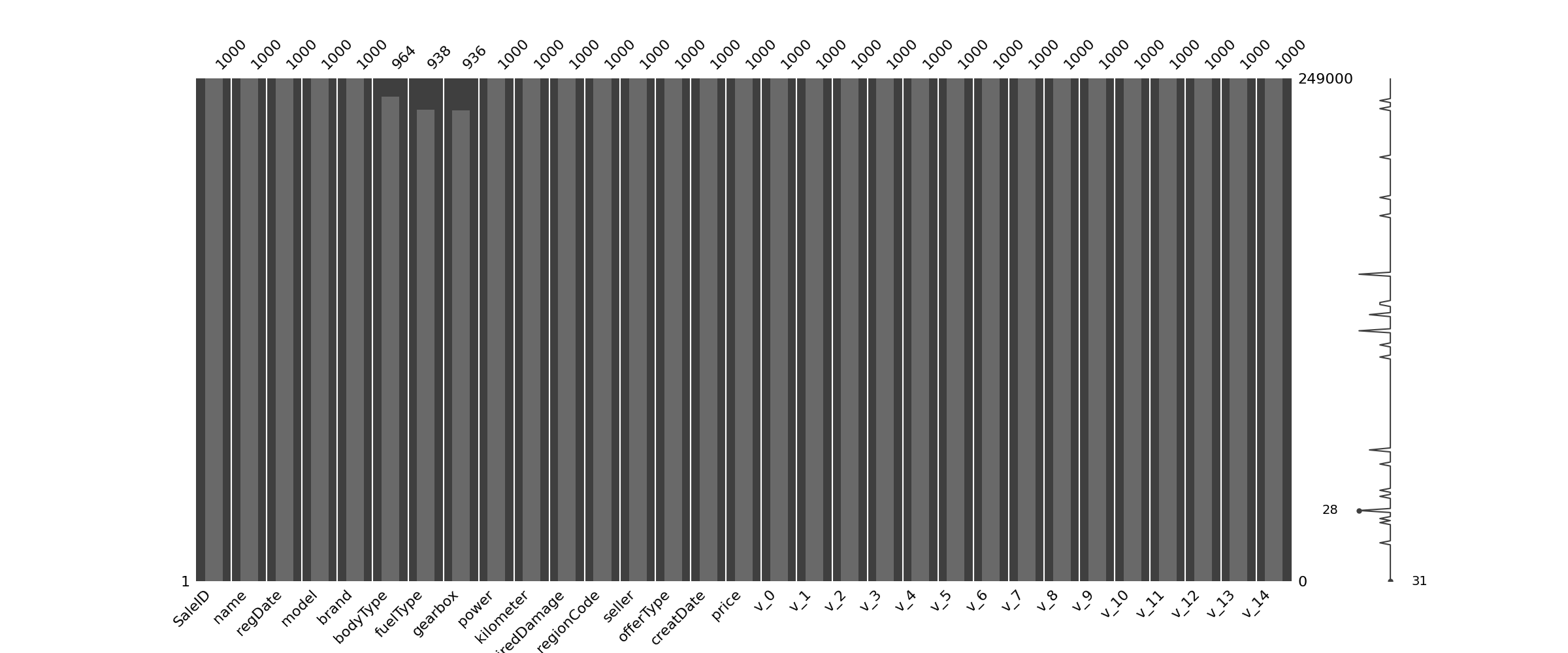
# msno.bar(Train_data.sample(1000)) # 条形图
# plt.show()
## 6)查看异常值检测
# Train_data.info()
## print(Train_data["notRepairedDamage"].value_counts()) # 返回包含值和count
Train_data["notRepairedDamage"].replace("-", np.nan, inplace=True) # 将数据中‘-’替换成nan值
# print(Train_data.isnull().sum())
#print(Train_data["notRepairedDamage"].value_counts())
#Test_data.info()
##print(Test_data["notRepairedDamage"].value_counts())
#Test_data["notRepairedDamage"].replace("-", np.nan, inplace=True)
##print(Test_data["notRepairedDamage"].value_counts())
# 删除严重倾斜的数据
#print(Train_data["seller"].value_counts())
#print(Train_data["offerType"].value_counts())
# print(Test_data["seller"].value_counts())
# print(Test_data["offerType"].value_counts())
del Train_data["seller"]
del Train_data["offerType"]
# print(Train_data.info())
# print(Train_data.shape)
#del Test_data["seller"]
#del Test_data["offerType"]
# 了解预测值的分布
# print(Train_data["price"])
# print(Train_data["price"].value_counts())
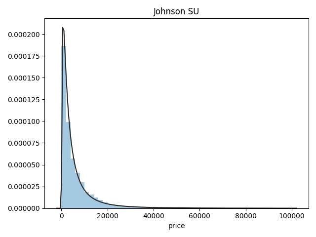
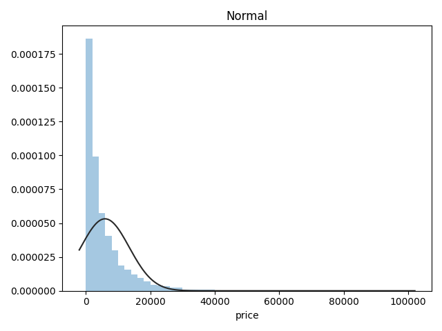
## 1)总体分布情况(无界约翰逊分布等)
import scipy.stats as st
# y = Train_data["price"]
# plt.figure(1); plt.title("Johnson SU") # 创建新图
# sns.distplot(y, kde=False, fit=st.johnsonsu)
# plt.figure(2); plt.title("Normal")
# sns.distplot(y, kde=False, fit=st.norm)
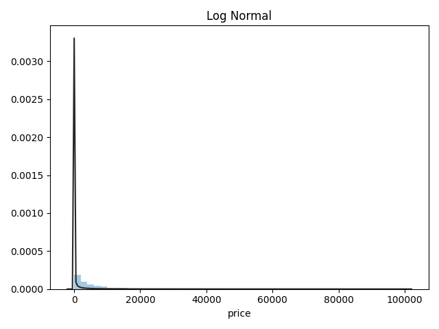
# plt.figure(3); plt.title("Log Normal")
# sns.distplot(y, kde=False, fit=st.lognorm)
# plt.show() # 最佳拟合是无界约翰逊分布
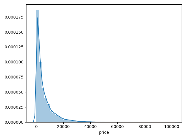
## 2)查看skewness and kurtosis
# sns.distplot(Train_data["price"])
# print("Skewness: %f" % Train_data["price"].skew()) # 偏度
# print("Kurtosis: %f" % Train_data["price"].kurt()) # 峰度
# plt.show()
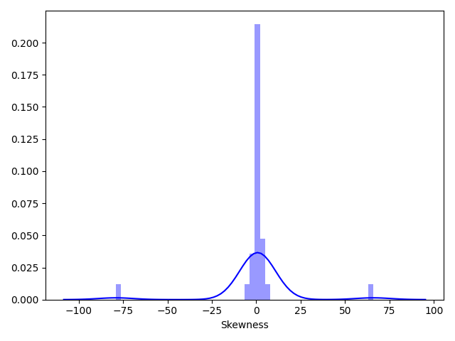
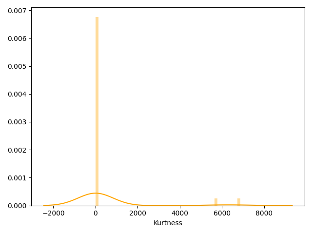
# print(Train_data.skew())
# print(Train_data.kurt())
# sns.distplot(Train_data.skew(), color="blue", axlabel="Skewness")
# plt.show()
# sns.distplot(Train_data.kurt(), color="orange", axlabel="Kurtness")
# plt.show()
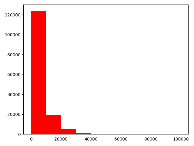
# 3)查看预测值的具体频数
# plt.hist(Train_data["price"], orientation="vertical", histtype="bar", color="red")
# plt.show() # 直方图
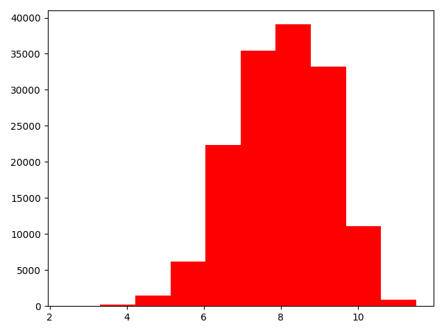
# log变换之后的分布比较均匀,可以进行log变换进行预测,这也是预测问题常用的trick
# plt.hist(np.log(Train_data["price"]), orientation="vertical", histtype="bar", color="red")
# plt.show()
## 查看特征
# 分离label即预测值
Y_train = Train_data["price"]
## 这个区别方式适用于没有直接label coding的数据
## 这里不适用,需要人为根据实际含义来区分
## 数字特征
## numeric_features = Train_data.select_dtypes(include=[np.number])
## numeric_features.columns
## # 类型特征
## categorical_features = Train_data.select_dtypes(include=[np.object])
## categorical_features.columns
# 数字特征
numeric_features = ['power', 'kilometer', 'v_0', 'v_1', 'v_2', 'v_3', 'v_4', 'v_5', 'v_6', 'v_7', 'v_8', 'v_9', 'v_10', 'v_11', 'v_12', 'v_13','v_14' ]
# 类别特征
categorical_features = ['name', 'model', 'brand', 'bodyType', 'fuelType', 'gearbox', 'notRepairedDamage', 'regionCode']
## 类别特征nunique分布——Train_data
# for cat_fea in categorical_features:
# print(cat_fea+"的特征分布如下:")
# print("{}特征有{}个不同的值".format(cat_fea, Train_data[cat_fea].nunique()))
# print(Train_data[cat_fea].value_counts())
## 类别特征nunique分布——Test_data
# for cat_fea in categorical_features:
# print(cat_fea+"的特征分布如下:")
# print("{}特征有{}个不同的值".format(cat_fea, Test_data[cat_fea].nunique()))
# print(Test_data[cat_fea].value_counts())
## 数字特征分析
numeric_features.append("price")
# print(numeric_features)
#print(Train_data.head())
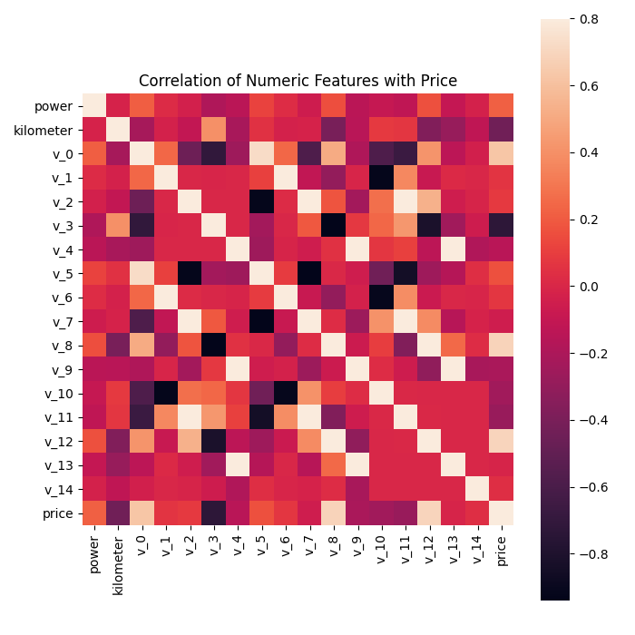
## 1)相关性分析
price_numeric = Train_data[numeric_features]
correlation = price_numeric.corr() # 返回一个相关系数的矩阵
# print(correlation["price"].sort_values(ascending=False),"\n") # 降序排序
# f , ax = plt.subplots(figsize = (7, 7))
# plt.title("Correlation of Numeric Features with Price")
# sns.heatmap(correlation, square=True, vmax=0.8) # 热图(显示相关系数)
# plt.show()
## 2)查看几个特征的偏度和峰度
# for col in numeric_features:
# print("{:15}".format(col),"Skewness:{:05.2f}".format(Train_data[col].skew()),
# " ",
# "Kurtosis:{:06.2f}".format(Train_data[col].kurt()))
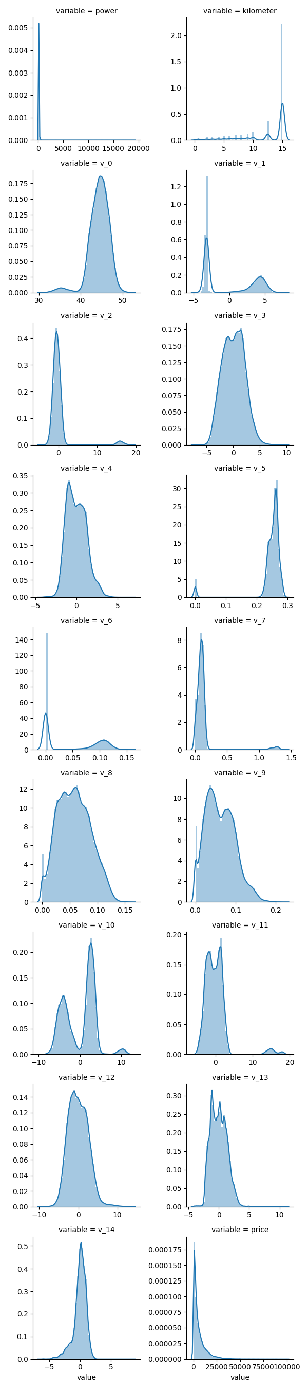
## 3)每个数字特征得分布可视化
# f = pd.melt(Train_data, value_vars=numeric_features) # 转换
# g = sns.FacetGrid(f,col="variable", col_wrap=2, sharex=False,sharey=False) # 以”variable“作“格子"绘图
# # plt.show()
# g = g.map(sns.distplot, "value") # 以”value“绘制到”格子”图中
# plt.show()
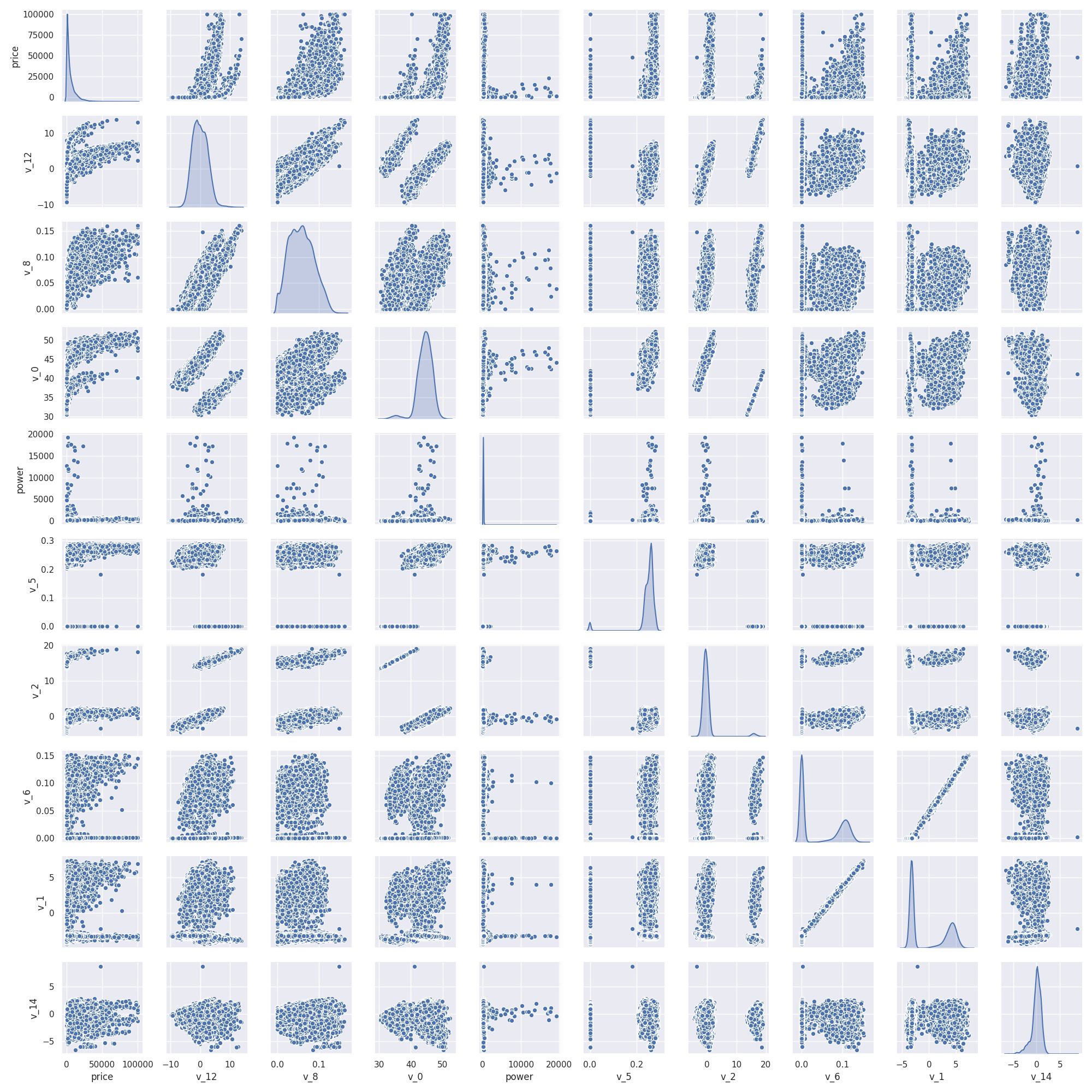
## 4)数字特征相互之间的关系可视化
# sns.set() # 风格设置
# colunms = ["price", "v_12", "v_8", "v_0", "power", "v_5", "v_2", "v_6", "v_1", "v_14"]
# sns.pairplot(Train_data[colunms],size=2, kind="scatter", diag_kind="kde") # 多变量图
# plt.show()
# print(Train_data.columns)
# print(Y_train)
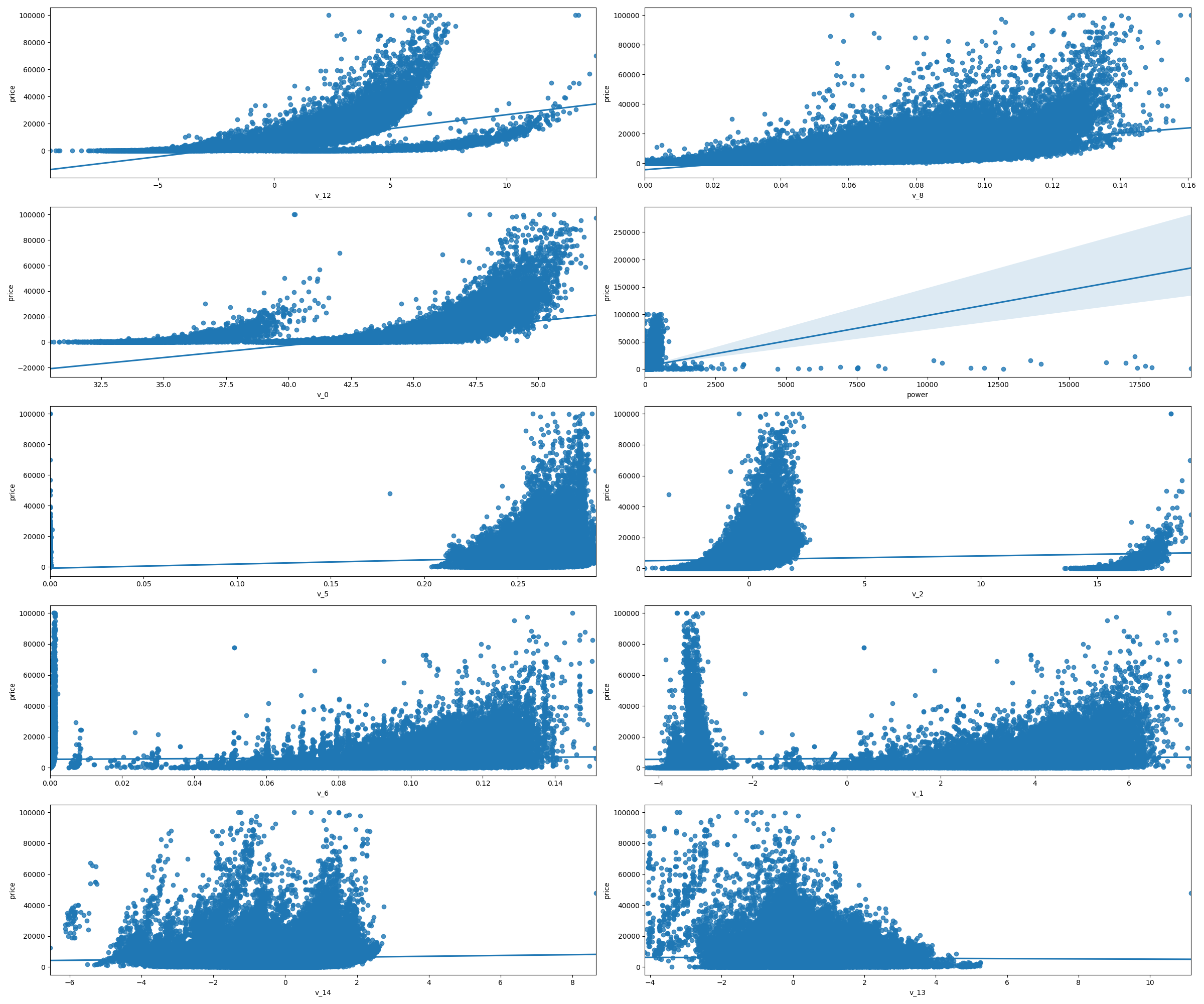
## 5)多变量互相关系回归关系可视化
# fig,((ax1, ax2), (ax3, ax4), (ax5, ax6), (ax7, ax8), (ax9, ax10)) = plt.subplots(nrows=5, ncols=2, figsize=(24, 20)) # 生成5行2列十个子图
# # ['v_12', 'v_8' , 'v_0', 'power', 'v_5', 'v_2', 'v_6', 'v_1', 'v_14']
# v_12_scatter_plot = pd.concat([Y_train,Train_data["v_12"]], axis=1) # 合并成一列
# #print(v_12_scatter_plot)
# sns.regplot(x="v_12", y="price", data=v_12_scatter_plot,scatter=True,fit_reg=True,ax=ax1) # 数据与回归模型拟合
#
# v_8_scatter_plot = pd.concat([Y_train,Train_data['v_8']],axis = 1)
# sns.regplot(x='v_8',y = 'price',data = v_8_scatter_plot,scatter= True, fit_reg=True, ax=ax2)
#
# v_0_scatter_plot = pd.concat([Y_train,Train_data['v_0']],axis = 1)
# sns.regplot(x='v_0',y = 'price',data = v_0_scatter_plot,scatter= True, fit_reg=True, ax=ax3)
#
# power_scatter_plot = pd.concat([Y_train,Train_data['power']],axis = 1)
# sns.regplot(x='power',y = 'price',data = power_scatter_plot,scatter= True, fit_reg=True, ax=ax4)
#
# v_5_scatter_plot = pd.concat([Y_train,Train_data['v_5']],axis = 1)
# sns.regplot(x='v_5',y = 'price',data = v_5_scatter_plot,scatter= True, fit_reg=True, ax=ax5)
#
# v_2_scatter_plot = pd.concat([Y_train,Train_data['v_2']],axis = 1)
# sns.regplot(x='v_2',y = 'price',data = v_2_scatter_plot,scatter= True, fit_reg=True, ax=ax6)
#
# v_6_scatter_plot = pd.concat([Y_train,Train_data['v_6']],axis = 1)
# sns.regplot(x='v_6',y = 'price',data = v_6_scatter_plot,scatter= True, fit_reg=True, ax=ax7)
#
# v_1_scatter_plot = pd.concat([Y_train,Train_data['v_1']],axis = 1)
# sns.regplot(x='v_1',y = 'price',data = v_1_scatter_plot,scatter= True, fit_reg=True, ax=ax8)
#
# v_14_scatter_plot = pd.concat([Y_train,Train_data['v_14']],axis = 1)
# sns.regplot(x='v_14',y = 'price',data = v_14_scatter_plot,scatter= True, fit_reg=True, ax=ax9)
#
# v_13_scatter_plot = pd.concat([Y_train,Train_data['v_13']],axis = 1)
# sns.regplot(x='v_13',y = 'price',data = v_13_scatter_plot,scatter= True, fit_reg=True, ax=ax10)
# plt.show()
# 类别特征分析
## 1)nunique分布
# for fea in categorical_features:
# print(Train_data[fea].nunique())
#
# print(categorical_features)
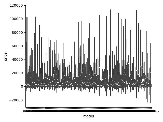
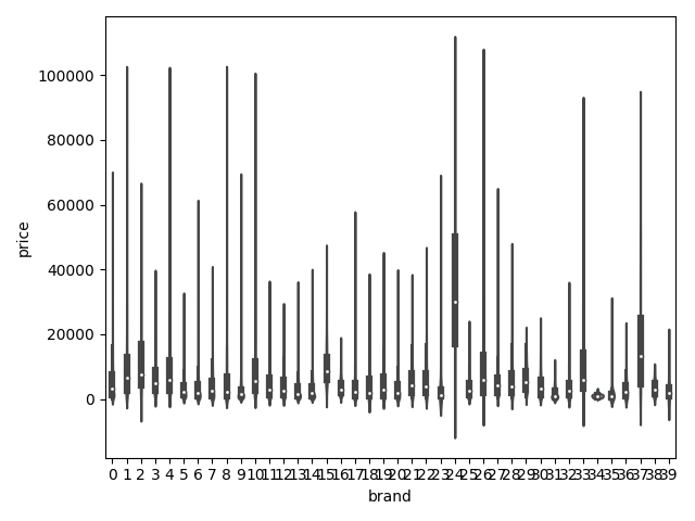
## 2)类别箱形图可视化
# 因为 name和 regionCode的类别太稀疏了,这里我们把不稀疏的几类画一下
categorical_features = ["model",
"brand",
"bodyType",
"fuelType",
"gearbox",
"notRepairedDamage"]
for c in categorical_features:
Train_data[c] = Train_data[c].astype("category") # 强制转换数据类型
if Train_data[c].isnull().any(): # 检查字段缺失
Train_data[c] = Train_data[c].cat.add_categories(["MISSING"]) # 添加新类别
Train_data[c] = Train_data[c].fillna("MISSING") # 填充为NAN的值
# def boxplot(x, y, **kwargs):
# sns.boxplot(x=x, y=y) # 箱形图
# x=plt.xticks(rotation=90) # 设置坐标轴
#
# f = pd.melt(Train_data, id_vars=["price"], value_vars=categorical_features)
# g = sns.FacetGrid(f,col="variable", col_wrap=2, sharex=False,sharey=False,size=5)
# g = g.map(boxplot, "value", "price")
# plt.show()
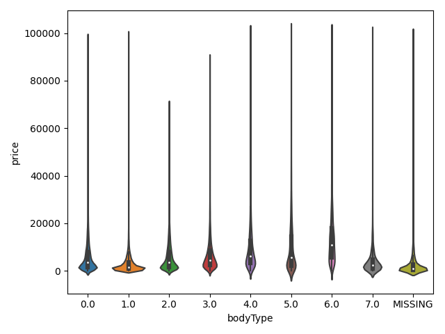
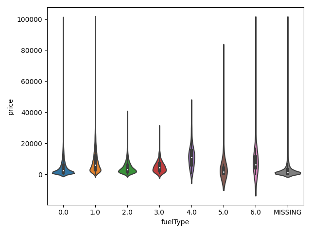
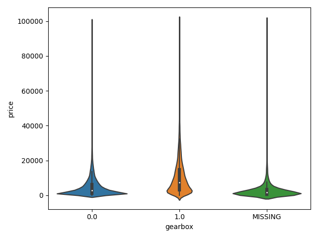
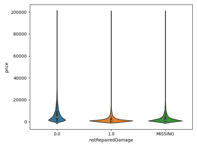
## 3)类别特征的小提琴图可视化
#print(Train_data.columns)
# catg_list = categorical_features
# target = "price"
# for catg in catg_list:
# sns.violinplot(x=catg,y=target,data=Train_data)
# plt.show()
# print(categorical_features)
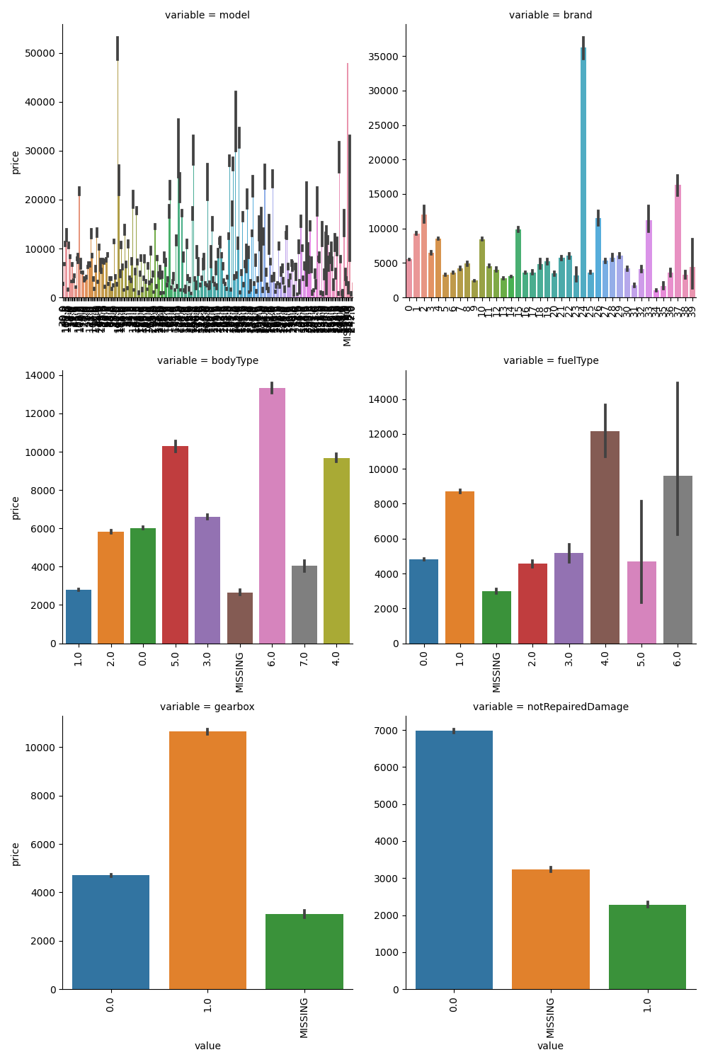
## 4)类别特征的柱形图可视化
# def bar_plot(x,y,**kwargs): # 柱形图
# sns.barplot(x=x,y=y)
# x=plt.xticks(rotation=90)
# f = pd.melt(Train_data, id_vars=["price"], value_vars=categorical_features)
# g = sns.FacetGrid(f, col="variable",col_wrap=2,sharex=False,sharey=False,size=5)
# g = g.map(bar_plot, "value", "price")
# plt.show()
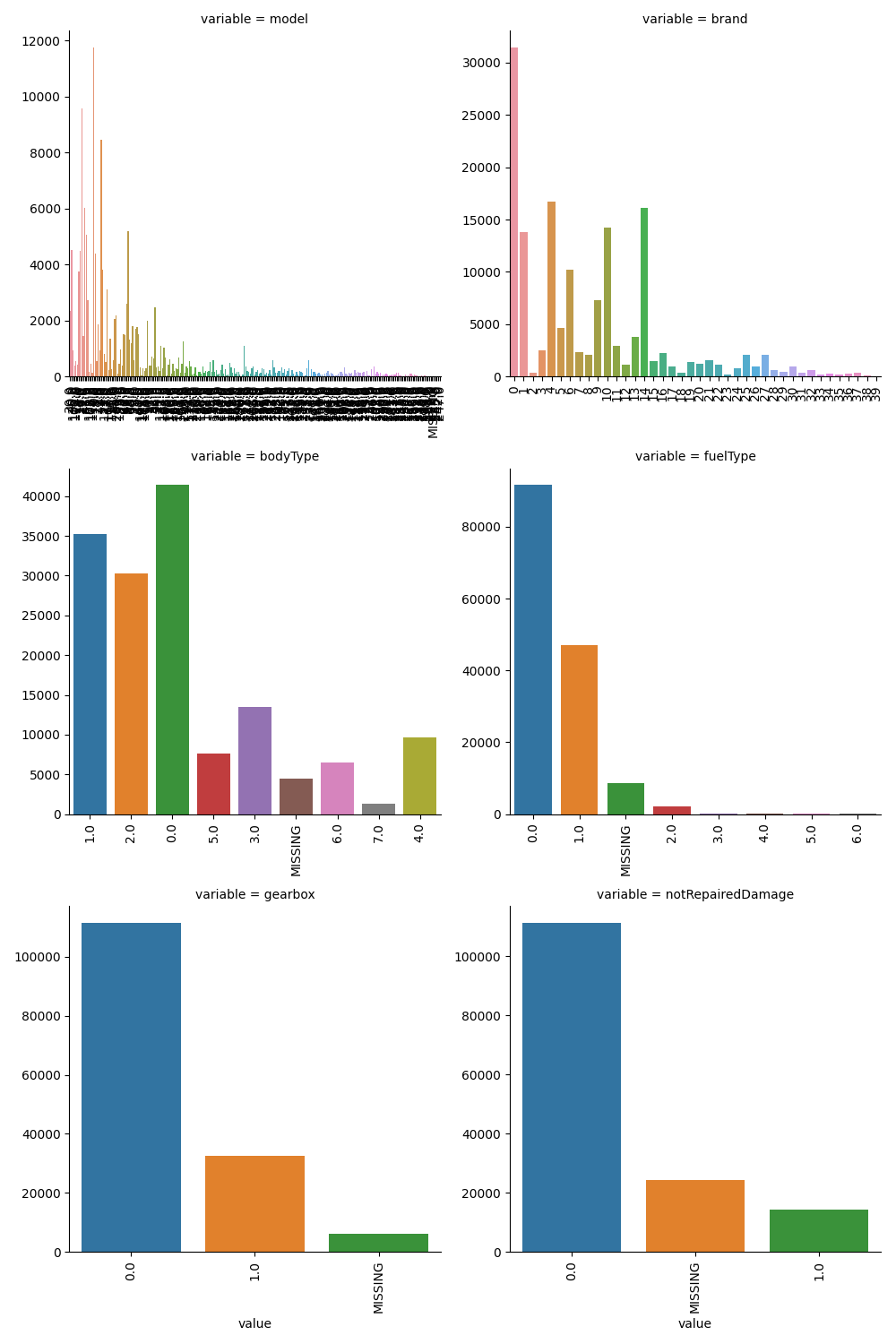
## 5)类别特征的每个类别频数可视化
# def count_plot(x,**kwargs): # 计数直方图
# sns.countplot(x=x)
# x=plt.xticks(rotation=90)
# f = pd.melt(Train_data,value_vars=categorical_features)
# g = sns.FacetGrid(f,col="variable", col_wrap=2,sharex=False,sharey=False,size=5)
# g = g.map(count_plot,"value")
# plt.show()
## 生成数据报告
import pandas_profiling
#
# pfr = pandas_profiling.ProfileReport(Train_data)
# pfr.to_file("./example.html")
|